Operating Systems (OS)
An Operating System (OS) is system software that manages computer hardware and software resources and provides common services for computer programs.
Think of it as the "manager" of your computer.
+---------------------+
|   Your Apps         |
| (Chrome, VS Code)   |
+----------+----------+
| Operating System    |
| (Windows, Linux, macOS) |
+----------+----------+
| Hardware            |
| (CPU, RAM, Disk, GPU) |
+---------------------+
Why Do We Need an OS?
| Problem | OS Solves It |
|---|---|
| Hardware is complex | OS hides complexity |
| Apps need CPU, RAM, disk | OS allocates fairly |
| Multiple apps run together | OS schedules them |
| You click mouse → app opens | OS translates input |
Without OS → You’d write machine code for every CPU instruction.
With OS → You just double-click an app.
Core Functions of an OS
| Function | What It Does | Example |
|---|---|---|
| Process Management | Create, run, kill apps | Open Chrome → new process |
| Memory Management | Give RAM to apps | 2GB to VS Code |
| File System Management | Read/write files | Save report.docx |
| Device Management | Talk to hardware | Print to printer |
| Security | Protect data/users | Login password |
| User Interface | GUI or CLI | Desktop, Terminal |
Types of Operating Systems
| Type | Examples | Use Case |
|---|---|---|
| Desktop OS | Windows, macOS, Linux (Ubuntu) | Laptops, PCs |
| Mobile OS | Android, iOS | Phones |
| Server OS | Ubuntu Server, Windows Server, RHEL | Cloud, data centers |
| Real-Time OS (RTOS) | FreeRTOS, VxWorks | Robots, cars |
| Embedded OS | Linux (Raspberry Pi), TinyOS | IoT devices |
Key Components of an OS
+---------------------+
|     User Space      |
|  Apps, Libraries    |
+----------+----------+
|     Kernel Space    |
|  [Kernel]           |
|  ├─ Process Mgr     |
|  ├─ Memory Mgr      |
|  ├─ File System     |
|  ├─ Device Drivers  |
|  └─ System Calls     |
+----------+----------+
|     Hardware        |
+---------------------+
Von Neumann Architecture
The Von Neumann Architecture is the foundational design of most modern computers, where a single memory stores both program instructions and data, and the CPU executes instructions in a fetch-decode-execute cycle.
+------------------+
|     Memory       | ← Stores BOTH Instructions & Data
| [1010] [Data]    |
+--------+---------+
         ↑
         |
       CPU
  +------+------+
  |  ALU  |     |
  |  Registers  |
  |  Control    |
  +-------------+
"Stored Program Concept" – Instructions and data are stored in the same memory and are indistinguishable in format.
Core Components
| Component | Full Name | Role | Details |
|---|---|---|---|
| 1. CPU | Central Processing Unit | Brain of the computer | Executes instructions using fetch-decode-execute cycle |
| 2. Memory | Main Memory (RAM) | Stores instructions + data | Single shared memory (Von Neumann bottleneck) |
| 3. I/O System | Input/Output Devices | Interact with user/world | Keyboard, screen, disk, network |
| 4. Bus System | Interconnect | Data highways | Connects CPU, Memory, I/O |
1. CPU (Central Processing Unit) – The Executor
+---------------------+
|        CPU          |
|  +---------------+  |
|  |  ALU          |  | ← Arithmetic Logic Unit (ADD, AND, etc.)
|  +---------------+  |
|  |  Control Unit |  | ← Orchestrates fetch-decode-execute
|  +---------------+  |
|  |  Registers     |  | ← High-speed storage (PC, IR, ACC, etc.)
|  +---------------+  |
+---------------------+
Sub-Components of CPU
| Part | Function |
|---|---|
| ALU | Performs math/logic (+, &, ==) |
| Control Unit | Sends control signals (e.g., "read memory") |
| Registers | Tiny, fast storage inside CPU |
2. Memory (RAM) – The Shared Workspace
Memory Address | Content
---------------|---------
0x1000         | LOAD R1, [0x2000]
0x1004         | ADD R1, R2
0x1008         | STORE R1, [0x2008]
0x2000         | 5        ← Data
0x2004         | 3        ← Data
- Stores both:
- Instructions (code)
- Data (variables)
- Random Access: Any location in ~same time
- Volatile: Lost on power off
3. I/O System – The Bridge to the World
| Device | Type | Example |
|---|---|---|
| Input | User → CPU | Keyboard, mouse, microphone |
| Output | CPU → User | Monitor, speaker, printer |
| Storage | Persistent | SSD, HDD, USB |
Disk → Memory → CPU → Screen
Bus System – The Data Highways
The Bus System is a set of parallel wires (physical or logical) that carry data, addresses, and control signals between CPU, Memory, and I/O.
CPU ↔ [Address Bus] ↔ Memory
CPU ↔ [Data Bus]    ↔ Memory
CPU ↔ [Control Bus] ↔ Memory/I/O
Three Types of Buses
| Bus Type | Direction | Width | Purpose | Example |
|---|---|---|---|---|
| Address Bus | CPU → Memory/I/O | 32/64 bits | "Where?" – Memory address to read/write | 0x2000 |
| Data Bus | Bidirectional | 32/64 bits | "What?" – Actual data/instruction | LOAD R1, R2 or 42 |
| Control Bus | Bidirectional | ~10–20 lines | "When/How?" – Control signals | READ, WRITE, IRQ |

Summary Table
| Component | Analogy | Key Role |
|---|---|---|
| CPU | Brain | Executes |
| Memory | Desk | Stores code + data |
| I/O | Hands/Eyes | Input/Output |
| Bus System | Roads | Connects everything |
Golden Rule:
"CPU asks Memory for instructions/data using Address Bus, gets them via Data Bus, and uses Control Bus to say READ/WRITE."
CPU Registers (The "Scratchpad")
| Register | Purpose | Example |
|---|---|---|
| PC (Program Counter) | Holds address of next instruction | 0x1000 |
| IR (Instruction Register) | Holds current instruction being executed | ADD R1, R2 |
| MAR (Memory Address Register) | Holds memory address to read/write | 0x2000 |
| MDR (Memory Data Register) | Holds data from/to memory | 42 |
| ACC (Accumulator) | Stores intermediate results | Result of ADD |
| General-Purpose Registers (R0–Rn) | Fast storage for variables | R1 = 10 |
| Status Register (Flags) | Stores condition codes | Z=1 (zero), N=1 (negative) |
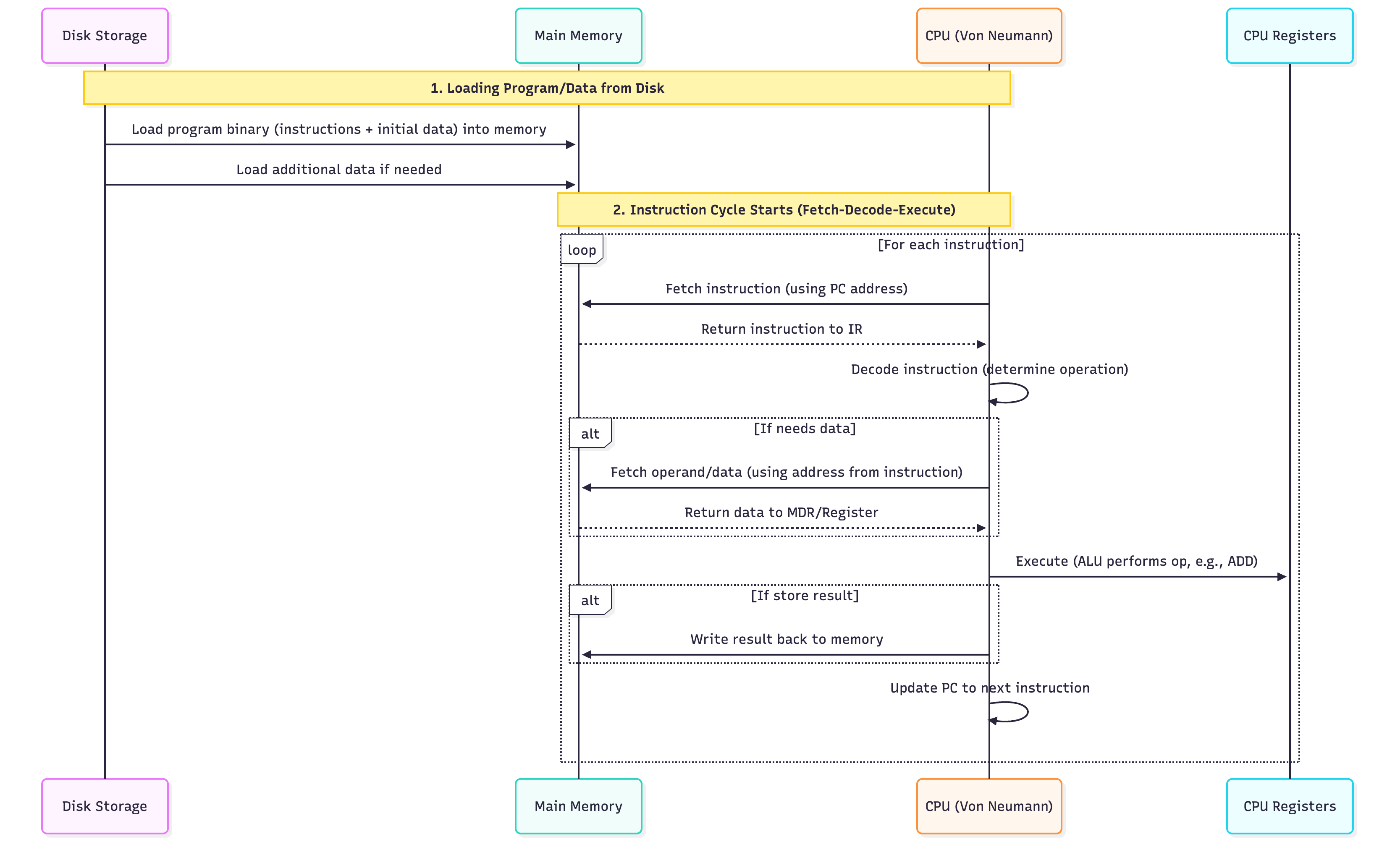
Instruction Cycle (Fetch-Decode-Execute)
REPEAT FOREVER:
  1. FETCH
     PC → MAR
     Memory[MAR] → MDR → IR
     PC = PC + 1

  2. DECODE
     Decode IR → know operation (ADD, LOAD, etc.)

  3. EXECUTE
     Do the operation (ALU, memory, I/O)
     Update flags if needed
Modes of Execution
| Mode | Privilege | Use |
|---|---|---|
| User Mode | Limited | Run apps (Chrome, VS Code) |
| Kernel/Supervisor Mode | Full access | OS kernel, drivers |
| Hypervisor Mode (modern) | Highest | Virtual machines (VMware, KVM) |
Switching: Apps use system calls → trap to kernel mode.
Example: Simple Program in Memory
Memory Address | Content
---------------|---------
0x1000         | LOAD R1, [0x2000]   ← PC points here
0x1004         | LOAD R2, [0x2004]
0x1008         | ADD R1, R2
0x100C         | STORE R1, [0x2008]
0x1010         | HALT
Data:
0x2000: 5
0x2004: 3
→ Result: 0x2008 = 8
Next: Want to see pipelining, interrupts, or real CPU (x86, ARM)?
Ask: "Explain CPU pipelining" or "How does an interrupt work?"
Process Management
1. What is a Program?
A program is a passive set of instructions stored on disk.
hello.c  →  Source
hello.exe → Executable (binary file on disk)
- No CPU, no memory
- Just a file
2. What is a Process?
A process is an active program in execution.
Program (on disk) → OS loads → Process (in RAM + CPU)
| Component | Meaning |
|---|---|
| Code (Text) | Instructions |
| Data | Global variables, heap, stack |
| Registers | PC, SP, CPU registers |
| State | Running, Ready, Blocked |
3. Process Control Block (PCB) – Process Attributes
PCB is the "ID card" of a process – OS stores all info here.
struct PCB {
    int pid;              // Process ID
    int state;            // Running, Ready, Blocked
    int priority;         // Scheduling priority
    void* pc;             // Program Counter
    void* registers[];    // CPU registers
    void* memory_limits;  // Base/limit
    list open_files;      // File descriptors
    int cpu_time_used;    // Total CPU used
    int arrival_time;     // When it arrived
    int burst_time;       // CPU needed
    // ... more
};
4. Process States (Lifecycle)
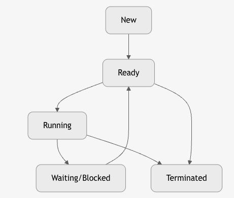
| State | Meaning |
|---|---|
| New | Just created, not in memory |
| Ready | In memory, waiting for CPU |
| Running | Executing on CPU |
| Waiting/Blocked | Waiting for I/O, signal |
| Terminated | Finished or killed |
5. Process Operations (System Calls)
| Operation | System Call | Action |
|---|---|---|
| Create | fork() |
Duplicate process |
| Execute | exec() |
Load new program |
| Wait | wait() |
Parent waits for child |
| Exit | exit() |
Terminate process |
| Kill | kill() |
Send signal |
pid_t pid = fork();     // Creates child
if (pid == 0) exec("ls"); // Child runs ls
6. Scheduling Queues
OS maintains queues of PCBs:
+-------------+     +-------------+     +-------------+
| Ready Queue | →   | Device Queue| →   | Job Queue   |
| (FCFS, RR)  |     | (Disk, Net) |     | (Batch)     |
+-------------+     +-------------+     +-------------+
| Queue | Contains |
|---|---|
| Job Queue | All processes in system |
| Ready Queue | Processes in RAM, ready for CPU |
| Device Queue | Processes waiting for I/O |
7. CPU Scheduler & Dispatcher
| Component | Role |
|---|---|
| Scheduler | Decides which process runs next |
| Dispatcher | Switches CPU to that process |
8. Context Switching
Saving state of current process → Loading state of next process
Process A (Running)
   ↓
Save: PCB_A (PC, registers, SP)
   ↓
Load: PCB_B
   ↓
Process B (Running)
Time: 1–100 μs (overhead)
9. CPU Scheduling Timings
| Term | Formula | Meaning |
|---|---|---|
| Arrival Time (AT) | - | When process enters system |
| Burst Time (BT) | - | CPU time needed |
| Completion Time (CT) | - | When process finishes |
| Turnaround Time (TAT) | CT - AT |
Total time in system |
| Waiting Time (WT) | TAT - BT |
Time spent waiting |
| Response Time (RT) | First CPU - AT | Time to first run |
10. Types of Schedulers
| Type | When | Goal |
|---|---|---|
| Long-term (Job) | Admit to RAM | Balance load |
| Mid-term | Swap in/out | Manage memory |
| Short-term (CPU) | Pick next process | Minimize wait |
11. Summary Diagram

12. Golden Rules
| Rule | Why |
|---|---|
| Process ≠ Program | One program → many processes |
| PCB = Process DNA | OS tracks everything here |
| Context switch = expensive | Save/restore registers |
| Scheduler = fairness + performance | FCFS, SJF, RR, Priority |
CPU Scheduling Algorithms**
Goal: Maximize CPU utilization, throughput, minimize waiting time, turnaround time, response time.
1. First-Come, First-Served (FCFS)
"Queue at the counter" – Non-preemptive
Avg WT = (0+20+22)/3 = 14
Cons: Convoy Effect – Short jobs wait behind long ones.
2. Shortest Job First (SJF) – Optimal (Non-Preemptive)
"Do small tasks first"
Cons: Starvation for long jobs, needs burst time prediction
3. Shortest Remaining Time First (SRTF) – Preemptive SJF
"If a shorter job arrives, pause current"
Same as SJF if no new arrivals during execution.
With new short job, it preempts.
4. Round Robin (RR) – Preemptive, Time-Sharing
"Everyone gets 1 turn" – Time Quantum (e.g., 4 ms)
Pros: Fair, responsive
Cons: High context switch overhead if quantum too small
5. Priority Scheduling
"VIPs go first" – Preemptive or Non-Preemptive
Cons: Starvation of low-priority jobs
Fix: Aging – Increase priority over time
6. Multilevel Queue Schedulers
Why?
| Problem | Solution |
|---|---|
| Different types of processes (interactive, batch, real-time) | Separate queues |
| Single algorithm not optimal for all | Tailored scheduling per queue |
| Starvation in priority | Feedback promotes/demotes |
"Fixed priority queues – processes stay in their queue."
+--------------------+
| Queue 0 (RR, q=8)  | ← System processes (Highest)
+--------------------+
| Queue 1 (RR, q=16) | ← Interactive (Foreground)
+--------------------+
| Queue 2 (FCFS)     | ← Batch (Background)
+--------------------+
| Feature | Detail |
|---|---|
| Fixed Assignment | Process enters one queue and stays |
| Queue Priority | Higher queue → always runs first |
| Intra-Queue Scheduling | Each queue has its own algorithm |
| No Movement | No promotion/demotion |
Pros & Cons
| Pros | Cons |
|---|---|
| Tailored scheduling | Starvation of lower queues |
| Simple | Inflexible |
| Predictable | Poor for dynamic workloads |
7. Multilevel Feedback Queue (MLFQ)
"Dynamic priority – processes move between queues based on behavior."
+--------------------+
| Q0 (RR, q=8)       | ← New / Short jobs
+--------------------+
| Q1 (RR, q=16)      | ← Used full quantum
+--------------------+
| Q2 (FCFS)          | ← CPU-bound (long jobs)
+--------------------+
Rules of MLFQ
| Rule | Meaning |
|---|---|
| 1 | If Priority(A) > Priority(B) → A runs |
| 2 | If Priority(A) == Priority(B) → Round-robin |
| 3 | New process → top queue |
| 4 | Uses full quantum → demote to next queue |
| 5 | After some time → promote to higher queue (aging) |
| 6 | I/O-bound → stays in high queue |
Queue Movement
| Time | Action |
|---|---|
| 0 | P1 in Q0 |
| 2 | P1 uses full quantum → demote to Q1 |
| 4 | P2 returns early → stays in Q0 |
| 8 | P1 in Q1, uses 2 → still 1 left |
But in real systems, MLFQ wins because short jobs finish fast.
Aging (Anti-Starvation)
Every 5 seconds:
  for each process in lower queue:
    priority++
Prevents infinite wait.
Real-World Use
| OS | Scheduler |
|---|---|
| Windows | MLFQ-inspired (priority + quantum) |
| Linux (2.6+) | CFS (fair share) – evolved from MLFQ |
| macOS | MLFQ with fairness |
| Unix | Original MLFQ |
MLFQ is the foundation of modern OS schedulers.
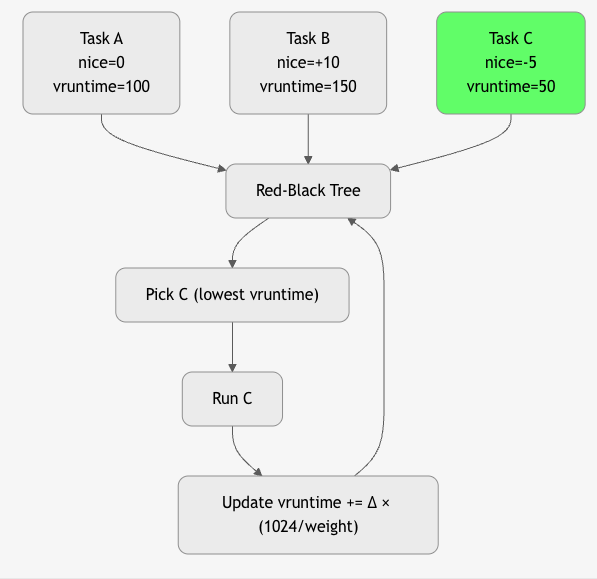
Linux CFS
CFS = Completely Fair Scheduler
Goal: Give every process a fair share of CPU time, proportional to its nice value.
- Replaced O(1) and earlier schedulers
- Default in Linux since 2007
- Used in Ubuntu, RHEL, Android, etc.
Core Idea: Virtual Runtime (vruntime)
"The process that has used the least CPU time runs next." "Every nanosecond of CPU is accounted for, and the task that has waited longest (in weighted time) runs to run."
vruntime = actual_runtime × (1024 / weight)
- Lower vruntime → higher priority
- Fairness = equal vruntime over time
Key Concepts
| Concept | Meaning |
|---|---|
| Nice Value | -20 (highest) to +19 (lowest) → default 0 |
| Weight | weight = 1024 / (1.25^nice) |
| Red-Black Tree | Stores runnable tasks sorted by vruntime |
| sched_latency | Target time slice (~20 ms for 4 tasks) |
| min_granularity | Minimum time quantum (~1 ms) |
Algorithm
Summary Table: CPU Scheduling
| Algorithm | Preemptive? | Avg WT (Example) | Best For |
|---|---|---|---|
| FCFS | No | 14 | Batch |
| SJF | No | 4 | Minimum wait |
| SRTF | Yes | ~4 | Optimal |
| RR | Yes | 2.67 | Interactive |
| Priority | Yes/No | Varies | Real-time |
| MLFQ | Yes | Balanced | General-purpose |
Inter-Process Communication (IPC)
IPC = How processes talk to each other
Process A        Process B
   ↓                ↓
[Shared Memory] OR [Message Passing]
1. Why IPC?
| Use Case | Example |
|---|---|
| Data Sharing | Web server → cache |
| Synchronization | Producer-Consumer |
| Modularity | Microservices |
2. Two Models of IPC
| Model | Mechanism | Speed | Example |
|---|---|---|---|
| Shared Memory | Same memory region | Fast | mmap, shmget |
| Message Passing | Send/Receive messages | Slower | Pipes, Sockets, MQ |
IPC Mechanisms
1. Pipes
Unidirectional data channel between related processes (parent-child).
- Anonymous: Created via pipe() → 2 file descriptors (read/write)
- Named (FIFO): mkfifo() → any process can open
Use: Shell pipelines (ls | grep), parent → child data
int pipefd[2];
pipe(pipefd);
write(pipefd[1], "hi", 2);  // Parent
read(pipefd[0], buf, 2);    // Child
- Anonymous Pipe: Parent → Child
- Named Pipe (FIFO): Any process
2. Message Queues
Kernel-persistent queue for structured messages.
- mq_open(), mq_send(), mq_receive()
- Messages have priority
- Survives process crash
Use: Decoupled communication, task queues
mqd_t mq = mq_open("/myqueue", O_CREAT);
mq_send(mq, "data", 4, 0);
mq_receive(mq, buf, size, &prio);
Pros: Decoupled, priority
3. Shared Memory
Fastest IPC: processes map same physical memory.
- shmget(), shmat()
- No kernel copy → zero-copy
- Requires synchronization (semaphore/mutex)
Use: High-performance data sharing (databases, video)
int shmid = shmget(key, 1024, IPC_CREAT);
char* data = shmat(shmid, NULL, 0);
strcpy(data, "Hello");
Fastest but needs synchronization
4. Semaphores
Semaphore – An integer variable used for synchronization and resource counting.
Supports two atomic operations:
- wait() (P): Decrement (block if 0)
- signal() (V): Increment (wake up waiter)
Types: - Binary Semaphore = 0 or 1 → acts like a lock - Counting Semaphore = N → allows N resources
Mutex vs Semaphore – Key Difference
| Feature | Mutex | Semaphore |
|---|---|---|
| Purpose | Mutual Exclusion (lock) | Synchronization + Counting |
| Ownership | Owned by one thread | No ownership (any thread can signal) |
| Value | Always 1 (binary) | Can be N (counting) |
| Use Case | Protect critical section | Control access to N resources |
| Example | pthread_mutex_lock() |
sem_wait(&empty) |
Mutex = "I own this lock"
Semaphore = "There are 5 slots available"
Producer-Consumer Problem
Problem:
One or more producers generate data → put in a bounded buffer
One or more consumers take data from buffer
Challenges: - Buffer overflow (producer too fast) - Buffer underflow (consumer too fast) - Race condition on buffer access
Solution Using 3 Semaphores
#define BUFFER_SIZE 10
int buffer[BUFFER_SIZE];
int in = 0, out = 0;

// Semaphores
sem_t empty;    // Counts empty slots (init = 10)
sem_t full;     // Counts full slots  (init = 0)
sem_t mutex;    // Binary lock for buffer access (init = 1)
Producer Code
void producer() {
    int item;
    while (1) {
        item = produce_item();

        sem_wait(&empty);    // Wait for empty slot
        sem_wait(&mutex);    // Lock buffer

        buffer[in] = item;   // Critical section
        in = (in + 1) % BUFFER_SIZE;

        sem_post(&mutex);    // Unlock
        sem_post(&full);     // Signal: one more full slot
    }
}
Consumer Code
void consumer() {
    int item;
    while (1) {
        sem_wait(&full);     // Wait for full slot
        sem_wait(&mutex);    // Lock buffer

        item = buffer[out];  // Critical section
        out = (out + 1) % BUFFER_SIZE;

        sem_post(&mutex);    // Unlock
        sem_post(&empty);    // Signal: one more empty slot

        consume_item(item);
    }
}
How Semaphores Solve It
| Semaphore | Initial | Role |
|---|---|---|
empty |
10 | Blocks producer if buffer full |
full |
0 | Blocks consumer if buffer empty |
mutex |
1 | Prevents race condition on in/out |
Summary: Semaphores in Producer-Consumer
empty → "How many slots are free?"
full  → "How many items are ready?"
mutex → "Only one at a time can touch buffer"
No overflow, no underflow, no race condition — guaranteed by atomic
wait()/signal()
5. Sockets
Bidirectional communication endpoint (local or network).
- UNIX Domain: Local (AF_UNIX) → fast, file-based
- TCP/UDP: Network (AF_INET)
Use: Client-server, microservices, distributed systems
// TCP
socket() → bind() → listen() → accept()
// OR
socket() → connect()
Used in networking, microservices
6. Signals
Asynchronous notification to a process.
- kill(pid, SIGUSR1) → send
- signal(SIGUSR1, handler) → receive
- Limited data (just signal number)
Use: Terminate, pause, custom events (SIGUSR1/SIGUSR2)
kill(pid, SIGUSR1);  // Send
signal(SIGUSR1, handler); // Receive
Asynchronous, limited data
5. Summary Table: IPC
| Method | Speed | Sync Needed? | Use Case |
|---|---|---|---|
| Shared Memory | Fastest | Yes | High perf |
| Message Queue | Medium | No | Decoupled |
| Semaphores | Fast | Yes (with shared mem) | Sync + resource counting (Producer-Consumer) |
| Pipes | Medium | No | Parent-Child |
| Sockets | Slower | No | Network |
| Signals | Fast | No | Notify |
Golden Rules
| Scheduling | IPC |
|---|---|
| SJF = min wait time | Shared memory = fastest |
| RR = fair for interactive | Use semaphore with shared mem |
| MLFQ = best of both | Message passing = safer |
# Concurrent Programming
Concurrent Programming is the practice of designing and writing programs that can execute multiple tasks at the same time, either by parallel execution on multiple CPU cores or by interleaving operations on a single core.
Sequential:
Task A → Task B → Task C

Concurrent:
Task A  ↘
         ↘  →  Result
Task B  ↗
- Thread: Lightweight execution unit in a process
- Process: Isolated program with own memory
- Critical Section: Code that must run atomically
Why Concurrent Programming?
| Need | Example |
|---|---|
| Speed | Video encoding on 8-core CPU |
| Responsiveness | Web server handles 1000 users |
| Resource Use | I/O + CPU overlap (download + process) |
| Real-World Modeling | Simulate traffic, users, sensors |
Concurrency vs Parallelism
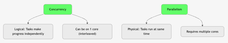
All parallel is concurrent, but not all concurrent is parallel. "Concurrency is about structure. Parallelism is about speed."
Models of Concurrent Programming
| Model | Language | Example |
|---|---|---|
| Threads | C, Java, Python | pthread_create(), Thread.start() |
| Async/Await | Python, JS, C# | async def fetch() |
| Actors | Erlang, Akka | actor ! message |
| Futures/Promises | Java, JS | CompletableFuture |
| Coroutines | Go, Kotlin | go func(), suspend fun |
Challenges & Solutions
| Challenge | Description | Solution(s) |
|---|---|---|
| Race Condition | Multiple tasks access shared data concurrently, leading to unpredictable outcomes depending on execution timing. | Mutex, Locks, Atomic operations |
| Deadlock | Two or more tasks permanently block each other by holding resources while waiting for others. | Avoid circular wait, Timeouts, Resource ordering |
| Starvation | A task is perpetually denied CPU or resources due to higher-priority tasks dominating. | Fair scheduling, Aging, Priority boosting |
| Livelock | Tasks actively retry conflicting actions indefinitely without progress (like deadlock but busy). | Randomized backoff, Leader election, Timeouts |
| Priority Inversion | A low-priority task blocks a high-priority one by holding a needed resource. | Priority inheritance, Priority ceiling |
| Overhead | High cost of context switching, synchronization, and thread management in concurrent programs. | Thread pools, Async I/O, Event-driven models |
Deadlock?
Deadlock = A set of processes are permanently blocked, each holding a resource and waiting for another resource held by another process in the set.
P1 holds R1 → wants R2
P2 holds R2 → wants R1
→ Circular wait → DEADLOCK
4 Necessary Conditions for Deadlock (Coffman Conditions)
| Condition | Meaning |
|---|---|
| 1. Mutual Exclusion | Resource can be held by only one process at a time |
| 2. Hold and Wait | Process holds resource while waiting for another |
| 3. No Preemption | Resources cannot be forcibly taken |
| 4. Circular Wait | Processes form a cycle in resource allocation graph |
All 4 must be true → deadlock possible
Break any one → deadlock impossible
1. Deadlock Prevention
Design system so that at least one of the 4 conditions is never satisfied.
1: Eliminate Mutual Exclusion
| How | Example |
|---|---|
| Use spooling instead of exclusive access | Printer → spool to disk → multiple jobs "share" |
| Not practical for most resources (RAM, files) |
Rarely used – most resources are inherently exclusive.
2: Eliminate Hold and Wait
| Method | How |
|---|---|
| Request all resources at once | Process declares all needs upfront |
| Release before requesting new | If can't get all, release held ones |
// Example
lock(R1, R2, R3);  // Get all or none
do_work();
unlock(R1, R2, R3);
Cons: - Low resource utilization - Starvation (long list of needs) - Hard to predict all needs
3: Allow Preemption
| How | Example |
|---|---|
| Force release of resource | OS kills process or takes resource |
| Checkpoint & rollback | Save state, restart later |
Used in: - Virtual memory (page stealing) - Some database systems
Cons: - Complex - Not all resources preemptible (printer half-printed)
4: Prevent Circular Wait → MOST PRACTICAL
| Method | How |
|---|---|
| Total ordering of resources | Assign number: R1=1, R2=2, ..., Rn=n |
| Request in increasing order | Process must acquire lower → higher |
// Correct
lock(R1);  // 1
lock(R3);  // 3

// Wrong → violates order
lock(R3);  // 3
lock(R1);  // 1 → DENIED or BLOCK
Pros: - Simple - No runtime overhead - Widely used
Cons: - Arbitrary ordering - May reduce concurrency
Prevention Summary Table
| Strategy | Breaks | Practical? | Used In |
|---|---|---|---|
| Mutual Exclusion | 1 | No | Spooling |
| Hold and Wait | 2 | Medium | Batch systems |
| No Preemption | 3 | Medium | VM, DB |
| Circular Wait | 4 | Yes | Most OS, DB, apps |
2. Deadlock Avoidance
Allow the system to enter unsafe states, but avoid deadlock using runtime checks.
Banker’s Algorithm (Dijkstra)
| Input | Meaning |
|---|---|
| Available | Free resources |
| Max | Max demand of each process |
| Allocation | Currently held |
| Need = Max – Allocation |
Safety Algorithm
- Find a process where Need ≤ Available
- Assume it finishes → add Allocation to Available
- Repeat
- If all finish → Safe, else Unsafe
Example:
Available: [3,3,2]
P1 Need: [1,0,2] → Safe → Run → Release
→ Available becomes [4,3,4]
Pros: Optimal utilization
Cons: Requires future knowledge, high overhead
Used in: Early systems, rarely in modern OS
3. Deadlock Detection
Allow deadlock to occur, then detect and recover.
Resource Allocation Graph (RAG)
graph TD
    P1 --> R1
    P2 --> R2
    R1 --> P2
    R2 --> P1
    style P1 fill:#f96
    style P2 fill:#f96
- Cycle = Possible deadlock
- Cycle + no preemption = Deadlock
Detection Algorithm
- Mark all processes with no outgoing request
- Remove them and their resources
- Repeat
- If any process remains → Deadlock
Run periodically or on resource request failure
4. Deadlock Recovery
Once detected, break the deadlock.
1: Process Termination
| Method | How |
|---|---|
| Kill one process | Choose cheapest (least CPU, memory) |
| Kill all | Restart system |
Cons: Lose work
2: Resource Preemption
| Steps |
|---|
| 1. Select victim process |
| 2. Rollback to safe state |
| 3. Preempt resource |
| 4. Allocate to waiting process |
Used in: Databases (transaction rollback)
Recovery Cost Factors
| Factor | Choose Victim By |
|---|---|
| CPU time used | Least |
| Resources held | Fewest |
| Processes to kill | Minimum |
| Priority | Lowest |
Real-World Example: Dining Philosophers
Philosopher i:
  think()
  pick_left_chopstick(i)
  pick_right_chopstick((i+1)%5)
  eat()
  put_down()
Deadlock: All pick left → wait for right → cycle
Prevention:
// Break circular wait
if (i == 4) {
  pick_right_first()
} else {
  pick_left_first()
}
Summary Table
| Method | When | Overhead | Practical |
|---|---|---|---|
| Prevention | Design time | Low | Yes (Circular wait) |
| Avoidance | Runtime | High | Rare |
| Detection | Periodic | Medium | Yes (with recovery) |
| Recovery | After deadlock | High | Yes (kill/restart) |
Best Practice in Modern Systems
| System | Strategy |
|---|---|
| Linux | Prevention (mutex order), Detection (hung task) |
| Databases | Detection + Transaction rollback |
| Java | ReentrantLock with tryLock() |
| Apps | Avoid nested locks, timeout, ordering |
Golden Rules
| Rule | Why |
|---|---|
| Always acquire locks in global order | Prevents circular wait |
Use try_lock() with timeout |
Avoids indefinite wait |
| Minimize lock scope | Reduces contention |
| Detect & recover | Better than crash |
Multithreading
Multithreading = Running multiple threads within one process.
Threads share memory, code, and file descriptors.
Process
├── Thread 1
├── Thread 2
└── Thread 3
    └── Shared: Heap, Code, Global Vars
Types of Threads
| Type | Managed By | Context Switch | Speed | Example |
|---|---|---|---|---|
| User-Level Threads (ULT) | User library | Fast (no kernel) | Very Fast | POSIX pthreads (early), Go goroutines |
| Kernel-Level Threads (KLT) | OS Kernel | Slow (kernel trap) | Slower | Linux (NPTL), Windows Threads |
| Hybrid (1:1 or M:N) | Both | Mixed | Balanced | Modern: Linux, Windows, Java |
1. User-Level Threads (ULT) – M:1 Model
Process
├── ULT1 → Scheduler (in user space)
├── ULT2 → Runs on one KLT
└── ULT3
| Pros | Cons |
|---|---|
| Fast context switch (no syscall) | Blocking call blocks all threads |
| Portable | No true parallelism |
| Low overhead | Kernel sees only one thread |
Example: Early Java Green Threads, Go (before 1.5)
2. Kernel-Level Threads (KLT) – 1:1 Model
Process
├── KLT1 → Kernel schedules
├── KLT2 → on CPU cores
└── KLT3
| Pros | Cons |
|---|---|
| True parallelism | Slow context switch |
| Non-blocking I/O | High overhead |
| Kernel scheduling |
Default in Linux (NPTL), Windows, macOS
3. Hybrid Threads (M:N Model)
Process
├── ULT1 → Mapped to KLT1
├── ULT2 → KLT1
├── ULT3 → KLT2
└── Scheduler (user + kernel)
| Pros | Cons |
|---|---|
| Best of both | Complex |
| Scalable (100K+ threads) | Harder to debug |
| Efficient |
Used in: - Go (goroutines → KLT) - Java (fibers, Project Loom) - Erlang (actors)
Multithreading vs Multiprocessing
| Feature | Multithreading | Multiprocessing |
|---|---|---|
| Execution Unit | Thread | Process |
| Memory | Shared | Isolated |
| Creation Cost | Low | High |
| Context Switch | Fast | Slow |
| Parallelism | Yes (on multi-core) | Yes |
| Fault Isolation | No (crash → whole process) | Yes |
| IPC | Direct (shared vars) | Pipes, sockets, queues |
| GIL (Python) | Blocked | Not blocked |
| Use Case | I/O-bound, shared data | CPU-bound, isolation |
When to Use What?
| Workload | Use |
|---|---|
| I/O-Bound (web server, DB) | Multithreading |
| CPU-Bound (ML, video encode) | Multiprocessing |
| Need Isolation (plugins) | Multiprocessing |
| Low Latency | Hybrid threads |
| Python | multiprocessing (bypass GIL) |
5. Real-World Examples
| App | Model |
|---|---|
| Nginx | Multithreading + event loop |
| Apache | Multiprocessing (prefork) |
| Chrome | One process per tab |
| Go Web Server | 100K goroutines (hybrid) |
| Python Flask | Multiprocessing for CPU |
6. Summary Table
| Feature | User Threads | Kernel Threads | Hybrid | Processes |
|---|---|---|---|---|
| Speed | Fastest | Slow | Fast | Slowest |
| Parallelism | No | Yes | Yes | Yes |
| Memory | Shared | Shared | Shared | Isolated |
| Blocking | All | One | One | One |
| Scalability | 1000s | 100s | 100K+ | 100s |
| Use | Legacy | Default | Modern | Isolation |
Golden Rules
| Rule | Why |
|---|---|
| Use threads for I/O, processes for CPU | Maximize performance |
| Avoid shared state | Prevent race conditions |
| Use thread pools | Reduce creation cost |
In Python: use multiprocessing for CPU |
Bypass GIL |
Memory Management
Memory management is the core OS function that allocates, tracks, protects, and reclaims memory for running programs. It ensures isolation, efficiency, and scalability by abstracting physical RAM into virtual address spaces.
1. Program Loading & Its Types
Program Loading = Process of transferring a program from disk to RAM and preparing it for execution.
Steps in Program Loading
- User invokes (e.g.,
./app,execve()syscall). - Loader reads executable file (ELF/PE format).
- Allocates virtual memory regions:
- Text (code) – read-only
- Data – initialized globals
- BSS – uninitialized (zero-filled)
- Heap – dynamic allocation
- Stack – local vars, function calls
- Loads segments into memory.
- Performs relocation (adjust addresses).
- Links libraries (static/dynamic).
- Sets PC (Program Counter) to entry point.
- Starts execution.
Types of Program Loading
| Type | Description | Pros | Cons | Use Case |
|---|---|---|---|---|
| Static Loading | Entire program + dependencies loaded at start | Fast startup, self-contained | Wastes memory, large binary | Embedded, small apps |
| Dynamic Loading | Modules loaded only when needed (lazy) | Saves memory, modular | Runtime delay | Large apps (Java, Python) |
| Absolute Loading | Fixed memory address | Simple | Inflexible | Bootloaders |
| Relocatable Loading | Base address assigned at load time | Flexible | Needs relocation | Most modern OS |
Example:
gcc -static app.c→ Static
python script.py→ Dynamic (imports loaded on demand)
2. Main Memory Management
Goal: Allocate physical RAM to processes efficiently.
Two main approaches:
A. Contiguous Allocation
Each process gets one continuous block of memory.
Allocation Strategies
| Strategy | How it Works | Pros | Cons |
|---|---|---|---|
| First Fit | First hole ≥ size | Fast | External fragmentation |
| Best Fit | Smallest hole ≥ size | Less waste | Slow search, tiny holes |
| Worst Fit | Largest hole | Leaves big holes | Often wasteful |
Fragmentation in Contiguous
- External: Free holes too small to use.
- Internal: Allocated block larger than needed.
Solution: Compaction (move processes) → expensive.
B. Non-Contiguous Allocation
Memory divided into fixed or variable units; process can span non-adjacent blocks.
3. Paging (Most Important – Non-Contiguous)
Paging = Divides memory into fixed-size pages (usually 4KB).
- Logical Address Space → divided into pages
- Physical Memory → divided into frames (same size)
Virtual Address:  [ Page Number | Page Offset ]
                   (p bits)     (f bits)
Page Table
Maps virtual page number → physical frame number
Page Table Entry (PTE):
| Valid Bit | Frame Number | Protection | Dirty | ...
Example
- 32-bit address, 4KB page → 20-bit offset, 12-bit page number
- 2^12 = 4096 pages → Page table has 4096 entries
- Each PTE = 4 bytes → Page table size = 16KB
Address Translation
Virtual Address: 0x12345678
→ Page Number: 0x1234
→ Page Offset: 0x5678

Page Table[0x1234] = Frame 0x9ABC
→ Physical Address = 0x9ABC5678
Multi-Level Paging (To Reduce Page Table Size)
Problem: 64-bit system → 2^52 pages → huge page table
2-Level Paging (32-bit)
Page Directory (PD) → Points to Page Tables (PT)
PT → Points to Frames
4-Level Paging (x86-64)
PML4 → PDPT → PD → PT → Frame
- Only used levels are allocated → sparse memory efficient
Translation Lookaside Buffer (TLB)
TLB = Cache of recent page table entries (in CPU)
- Hit: 1–2 cycles
- Miss: Page walk (100+ cycles)
CPU → TLB → Hit? → Physical Address
         ↓ Miss
     Page Walk (MMU) → Load PTE → TLB
- TLB Shootdown: On context switch or page invalidation → flush TLB.
Paging with Hashing (Hashed Page Table)
For 64-bit systems with sparse addresses.
- Hash(Virtual Page Number) → Hash Table Entry
- Handles huge address space efficiently.
4. Segmentation
Segmentation = Divides memory into variable-sized segments based on logical structure.
| Segment | Purpose |
|---|---|
| Code | .text |
| Data | .data, .bss |
| Stack | Local vars |
| Heap | Dynamic |
Segment Table
Segment Base | Limit | Protection
- Address:
[Segment Number | Offset] - Offset < Limit → Valid
Pros
- Logical division
- Easy sharing (e.g., shared library segment)
Cons
- External fragmentation
- Complex management
5. Segmentation + Paging (Paged Segmentation)
Best of both: Logical segments + fixed pages.
Segment Table → Points to Page Table
Page Table → Points to Frames
- Used in some older systems (e.g., Multics)
- Modern OS prefer pure paging (simpler)
Summary Table
| Concept | Type | Fragmentation | Table Overhead | Use Case |
|---|---|---|---|---|
| Contiguous | Single block | External + Internal | None | Simple systems |
| Paging | Fixed pages | Only Internal | Page Table | All modern OS |
| Segmentation | Variable | External | Segment Table | Logical structure |
| Paged Seg. | Hybrid | Internal | Two tables | Legacy |
Key Advantages of Paging (Why It's Dominant)
| Feature | Benefit |
|---|---|
| No external fragmentation | Any free frame can be used |
| Easy swapping | Fixed size → easy disk mapping |
| Sharing | Same frame mapped in multiple processes |
| Protection | Per-page R/W/X bits |
| Demand loading | Load page only on access |
Golden Rules
| Rule | Why |
|---|---|
| Paging > Segmentation | Simpler, no external frag |
| TLB is critical | 90%+ translations from TLB |
| Multi-level paging saves space | Only allocate used tables |
| Page size = 4KB (trade-off) | Balance internal frag vs table size |
Virtual Memory & Demand Paging
It allows programs to run as if they have more memory than physically available, enables process isolation, and supports efficient memory sharing.
Virtual Memory = An abstraction that gives each process the illusion of a large, private, contiguous memory space, even when physical RAM is limited.
Process A sees: 0x00000000 → 0xFFFFFFFFFFFFFFFF (16 EB)
Process B sees: Same range
→ But they are isolated and mapped to different physical RAM
Key Goals of Virtual Memory
| Goal | How Achieved |
|---|---|
| Large Address Space | 64-bit → 2^64 bytes (16 exabytes) |
| Process Isolation | Each process has private virtual space |
| Memory Protection | Per-page R/W/X permissions |
| Efficient Sharing | Shared libraries, IPC |
| Transparent Execution | Program runs without knowing physical limits |
Virtual vs Physical Address Space
| Virtual Address | Physical Address | |
|---|---|---|
| Seen by | Process | OS, Hardware |
| Range | 0 to 2^n-1 (e.g., 2^64) | 0 to actual RAM size |
| Translation | Via Page Table | Direct to RAM |
How Virtual Memory Works
Paging is the foundation of virtual memory.
- Memory divided into fixed-size pages (usually 4KB).
- Virtual Address =
[Page Number | Page Offset]
64-bit Virtual Address:
+--------------------------------------------------+
|  PML4 (9) | PDPT (9) | PD (9) | PT (9) | Offset (12) |
+--------------------------------------------------+
- Physical Memory = divided into frames (same size).
- Page Table maps virtual page → physical frame.
Demand Paging – "Load Only When Needed"
Demand Paging = Pages are loaded from disk into RAM only when accessed (on a page fault).
Why Demand Paging?
- Most programs don’t use all memory at once.
- Startup faster (don’t load entire binary).
- More processes can run (only active pages in RAM).
Page Fault Handling – Step by Step
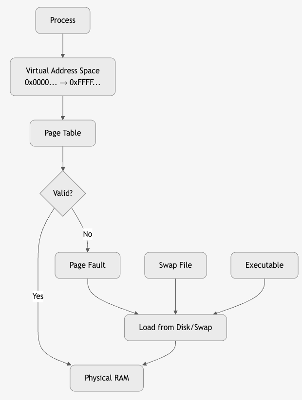
Valid/Invalid Bit in Page Table
| Bit | Meaning |
|---|---|
| 1 (Valid) | Page is in RAM |
| 0 (Invalid) | Page not in RAM → Page Fault |
4. Backing Store (Swap Space)
Swap File/Swap Partition on disk stores pages evicted from RAM.
# Linux
swapon /swapfile
free -h
# → Swap: 8GB
- Executable pages: Loaded from original binary (e.g.,
/bin/ls). - Anonymous pages (heap, stack): Saved to swap.
5. Page Replacement Algorithms
When RAM is full, OS evicts a page to make room.
| Algorithm | How | Pros | Cons |
|---|---|---|---|
| FIFO | First In, First Out | Simple | Belady's Anomaly |
| LRU | Least Recently Used | Good locality | Expensive (stack or counter) |
| Optimal | Replace page not used longest in future | Best (theoretical) | Impossible |
| Clock (Second Chance) | Circular list + reference bit | Efficient approximation | Moderate |
Key Metrics
| Metric | Meaning |
|---|---|
| Page Fault Rate | Faults per second |
| Major Fault | Requires disk I/O |
| Minor Fault | Page already in RAM (reclaim) |
| Working Set | Pages actively used |
Golden Rules
| Rule | Why |
|---|---|
| Demand paging = efficiency | Don’t load unused code |
| Page size = 4KB (sweet spot) | Balance frag vs table size |
| COW = fast fork | Share until write |
| Avoid thrashing | Monitor working set |
| TLB + Cache = speed | 99% translations from cache |
Thrashing
Thrashing = A severe performance degradation in a virtual memory system where the CPU spends more time handling page faults (swapping pages in/out of disk) than executing actual program instructions.
CPU Utilization: 90% → 10% → 1%
Page Fault Rate: 100/sec → 10,000/sec → 100,000/sec
→ System becomes unresponsive
Why Does Thrashing Happen?
Root Cause: Insufficient Physical RAM
- Too many processes → Total working set > Physical RAM
- OS keeps evicting pages to make room
- Evicted pages are immediately needed again
- → Endless page faults
graph LR
    A[Too Many Processes] --> B[Working Set > RAM]
    B --> C[Frequent Page Faults]
    C --> D[OS Evicts Pages]
    D --> E[Pages Needed Again]
    E --> C
    style C fill:#f96,stroke:#333
Working Set of a process = Set of pages it references in a time window (e.g., last 10 million instructions).
| Process | Working Set Size |
|---|---|
| Firefox | 200 MB |
| VS Code | 150 MB |
| Database | 500 MB |
Total RAM = 1 GB
3 processes → 850 MB working set → Fits → Smooth
5 processes → 1.5 GB working set → Thrashing
Thrashing in Action – Step-by-Step
Time 0:
  RAM: [P1 pages] [P2 pages] [P3 pages] → Full

Time 1:
  P4 starts → Needs 200 MB
  OS evicts P1's pages → P4 loads

Time 2:
  P1 runs → Page fault! → Evict P2 → Load P1
  P2 runs → Page fault! → Evict P3 → Load P2
  P3 runs → Page fault! → Evict P4 → Load P3

→ CPU busy with page faults, not work
Symptoms of Thrashing
| Symptom | How to Observe |
|---|---|
| High CPU usage by kernel | top → %sy (system) > 80% |
| High disk I/O | iostat → high kB_read/s, kB_wrtn/s |
| Low CPU utilization for user apps | %us < 5% |
| Unresponsive system | GUI freezes, commands lag |
| High page fault rate | vmstat → pgfault > 10,000/sec |
# Monitor
vmstat 1
# → si/so: swap in/out (high = bad)
# → bi/bo: blocks in/out

sar -B 1
# → pgpgin/s, pgpgout/s
Page Fault Types
| Type | Meaning |
|---|---|
| Minor Fault | Page in RAM (but not mapped) → fast |
| Major Fault | Page on disk → slow (10ms) |
| Thrashing = Too many major faults |
Belady’s Anomaly & Thrashing
With FIFO replacement, increasing frames can increase page faults → worsens thrashing.
Reference string: 1,2,3,4,1,2,5,1,2,3,4,5
3 frames → 9 faults
4 frames → 10 faults ← Anomaly
How OS Detects Thrashing
| Method | How |
|---|---|
| Page Fault Frequency (PFF) | If faults/sec > threshold → thrashing |
| CPU Utilization Drop | If CPU < 10% but faults high → suspend processes |
| Working Set Estimation | Track referenced pages over time |
Solutions to Prevent/Recover from Thrashing
- Increase Physical RAM
-
Best fix: Add more RAM or use faster storage (SSD).
-
Reduce Multiprogramming Degree
-
Suspend/Swap out processes until working sets fit.
-
Improve Locality
- Optimize code: Reduce random access, use arrays sequentially.
-
Compiler: Better loop ordering.
-
Priority-Based Swapping
-
Swap out low-priority or idle processes first.
-
Working Set Model (Theoretical)
- OS tracks working set window (Δ).
- If working set > RAM → suspend process.
Use Local Replacement (not Global) - Each process has fixed frame allocation. - Prevents one process from stealing all frames.
Linux Thrashing Protection
| Feature | How it Works |
|---|---|
| OOM Killer | Kills high-memory processes when swap exhausted |
| PSI (Pressure Stall Information) | Monitors memory pressure (some/full) |
| Swappiness | Controls swap aggressiveness (vm.swappiness=60) |
Real-World Example
Laptop: 8GB RAM
Running: Chrome (50 tabs) + VS Code + Docker + Zoom
→ Working set = 12GB
→ Thrashing: Disk LED blinking, UI freezes
→ Fix: Close Chrome tabs or add RAM
Golden Rules to Avoid Thrashing
| Rule | Why |
|---|---|
| Keep working set < RAM | Core principle |
| Monitor PSI / vmstat | Early detection |
| Use SSD, not HDD | 100x faster page faults |
| Set swappiness low | Prefer RAM over swap |
| Limit containers | Prevent memory explosion |
File System & Disk Management**
File systems and disk management are core OS components that organize, store, retrieve, and protect data on storage devices. They abstract raw disk blocks into user-friendly files and directories, while ensuring performance, reliability, and security.
1. What is a File?
File = A named collection of related data stored on disk.
File Attributes:
- Name: report.pdf
- Type: PDF
- Size: 2.1 MB
- Location: /home/user/docs/
- Permissions: rw-r--r--
- Timestamps: Created, Modified, Accessed
- Owner: user
File Types
| Type | Example |
|---|---|
| Regular | document.txt, image.jpg |
| Directory | folder/ |
| Symbolic Link | link → /real/path |
| Device | /dev/sda (block), /dev/tty (char) |
| Socket/Pipe | IPC |
2. File System – The Big Picture
File System = Software + Data Structures that manage how files are stored, organized, and accessed on a storage device.
3. Key File System Operations
| Operation | System Call | Action |
|---|---|---|
| Create | open("file", O_CREAT) |
Allocate inode + directory entry |
| Read | read(fd, buf, size) |
Copy from disk to memory |
| Write | write(fd, buf, size) |
Copy to disk (buffered) |
| Delete | unlink("file") |
Remove directory entry, free inode |
| Open | open() |
Get file descriptor |
| Close | close() |
Release fd |
| Seek | lseek() |
Move file pointer |
4. File System Structure on Disk
+---------------------+
| Boot Block          | ← Bootloader (optional)
+---------------------+
| Superblock          | ← FS metadata (size, inodes, blocks)
+---------------------+
| Inode Table         | ← File metadata (size, blocks, perms)
+---------------------+
| Data Blocks         | ← Actual file content
+---------------------+
5. Inode – The Heart of File Metadata
Inode = Index Node – Stores all file metadata except name.
struct inode {
    mode_t     mode;        // Permissions + type
    uid_t      uid;         // Owner
    gid_t      gid;         // Group
    off_t      size;        // Size in bytes
    time_t     atime;       // Access time
    time_t     mtime;       // Modify time
    time_t     ctime;       // Change time
    blkcnt_t   blocks;      // Number of blocks
    blkptr_t   block[15];   // Pointers to data blocks
};
Inode Block Pointers (EXT2/3/4)
12 Direct → 4KB blocks
1 Indirect → 1024 direct pointers
1 Double Indirect → 1024 indirect
1 Triple Indirect → 1024 double
→ Max file: ~2TB
6. Directory Structure
Directory = A special file containing (name, inode) pairs.
Directory Entry:
+--------+----------+
| Name   | Inode #  |
+--------+----------+
| .      | 2        |
| ..     | 2        |
| file.txt | 156      |
| docs/  | 789      |
+--------+----------+
- Hard Link: Multiple names → same inode
- Symbolic Link: File containing path to target
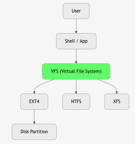
7. Disk Management – Partitioning & Formatting
1. Partitioning
Divides disk into logical sections.
# MBR (Legacy)
Partition 1: /boot (ext4)
Partition 2: / (ext4)
Partition 3: swap

# GPT (Modern)
GUID Partition Table → Up to 128 partitions
Tools: fdisk, gdisk, parted
2. Formatting
Installs file system on partition.
mkfs.ext4 /dev/sda1
mkfs.ntfs /dev/sdb1
8. Popular File Systems
| FS | OS | Features | Use Case |
|---|---|---|---|
| EXT4 | Linux | Journaling, extents, 1EB max | Default Linux |
| XFS | Linux | High perf, 8EB | Servers, big files |
| Btrfs | Linux | Snapshots, RAID, CoW | Advanced |
| NTFS | Windows | ACLs, encryption | Windows |
| APFS | macOS | Snapshots, encryption | macOS/iOS |
| FAT32 | Cross | Simple, 4GB file limit | USB drives |
9. Journaling – Crash Recovery
Journal = Log of pending operations before commit.
Write Intent → Journal → Commit → Data Blocks
→ If crash → Replay journal
Types: - Data Journaling: Log data + metadata (slow, safe) - Metadata Journaling: Log metadata only (fast) – EXT3/4 default - Ordered: Write data first, then metadata
10. File System Mounting
Mount = Attach file system to directory tree.
mount /dev/sda1 /home
# → /home now accesses sda1
/ (root)
├── home/
│   └── user/ ← /dev/sda1
├── boot/
└── etc/
Unmount: umount /home
11. Virtual File System (VFS) – Abstraction Layer
VFS = Unified interface for all file systems.
struct file_operations {
    ssize_t (*read) (struct file *, char *, size_t, loff_t *);
    ssize_t (*write) (struct file *, const char *, size_t, loff_t *);
    // ...
};
- Allows
ls,catto work on EXT4, NTFS, NFS, procfs
12. Disk Scheduling Algorithms
Optimize disk head movement to reduce seek time.
| Algorithm | How | Pros | Cons |
|---|---|---|---|
| FCFS | First come, first served | Simple | High seek |
| SSTF | Shortest Seek Time First | Low seek | Starvation |
| SCAN (Elevator) | Sweep head → reverse | Fair | |
| C-SCAN | Circular SCAN | More uniform | |
| LOOK | SCAN but stop at last request | Efficient |
13. RAID – Disk Redundancy & Performance
| Level | Min Disks | Features |
|---|---|---|
| RAID 0 | 2 | Striping → Speed |
| RAID 1 | 2 | Mirroring → Redundancy |
| RAID 5 | 3 | Striping + Parity → Balance |
| RAID 6 | 4 | Double parity → 2-disk fail |
| RAID 10 | 4 | Mirror + Stripe → Best |
14. Disk Caching & Buffering
- Page Cache: RAM cache of disk blocks
- Write-Back: Delay writes → coalesce
- Write-Through: Immediate write
Summary Diagram
Golden Rules
| Rule | Why |
|---|---|
| Inode ≠ Name | Name in directory, metadata in inode |
| Journaling saves data | Recover from crash |
| VFS = portability | Same API for all FS |
| Use SSD + EXT4 | Best performance |
| Backup > RAID | RAID ≠ backup |